Demonstration Procedure for GreG capabilities

All commands given here are followed by a comment area (after the exclamation mark !) in which a number refers to the detailed explanation after the text of the procedure. Comment lines are also in the body of the procedure for clarity.

!
! Basic plot : a simple curve
DEVICE XLANDSCAPE WHITE                      !1
SET PLOT LANDSCAPE                           !2
SET FONT SIMPLEX                             !3
COLUMN X 1 Y 2/FILE  GAG_DEMO:GREG1.TST      !4
LIMITS                                       !5
BOX                                          !6
LABEL "Offset frequency (s\\U-1\\D)"/X       !7
LABEL "Signal strength (Jy)"/Y               !8
CONNECT                                      !9
!
! More difficult: Markers and Errorbars
CLEAR PLOT                                   !10
LIMITS -50 50 * *                            !11
SET MARKER 4 1 .1                            !12
POINTS                                       !13
CURVE                                        !14
COLUMN Z 3                                   !15
ERRORBAR Y                                   !16
LABEL "Offset frequency (s\\U-1\\D)"/X       !17
LABEL "Signal strength (Jy)"/Y               !18
SET CENTERING 5                              !19
DRAW TEXT 0.0000E+00 10.70 "Demonstration of GREG : Curve and Errorb-
ars"/USER                                    !20
!
HARDCOPY/PLOT                                !21

1.

  First, define the graphic support to which you want to send all graphic output. Here this is an X-Window terminal in landscape mode, with white background: a new window with the title <GREG will appear. Note that it is not necessary to define a graphic support to begin drawing data. You may define (or change) your graphic support at any moment during the session without losing your plot.

2.

Specify the plot page has a ``landscape'' aspect (30 by 21 cm).

3.

Specify the character font is the simplex one (the faster to plot).

 

4.

Then read your data. The data file has a ``Table''-like organisation one column describes all the values of a given variable for all the data points, while one line contains the values of all the variables for a given data point. You can access any part of the input table. The data is read in list-directed format, so that values must be written in formatted way, with spaces, tabs or commas as separators. Here, the X value is read in column 1 (the Y value in column 2) from lines 4 to 30 of the input file GAG_DEMO:GREG1.TST. GAG_DEMO: is a logical name translated to a directory path by the software, so that GAG_DEMO:GREG1.TST will be expanded to something like /users/soft/gag/demo/greg1.tst.

 

5.

Define the values of the X and Y coordinates at the corners of the plot window. Here, the automatic setting is used; it computes extrema of X and Y values, then add some 10 percent margin to get the plot limits. LIMITS is a very fundamental command, because it defines the conversion formula between the user coordinates and the physical coordinates. As GreG almost always plots in User coordinates, no plot action should be issued before command LIMITS.

 

6.

Draw labelled axis around the plot window. This is useful in any plot, but contrary to LIMITS, this command is not compulsory. It can be issued at any moment (after LIMITS of course).

 

7.

Write the caption of the X axis, in particular the type and units of the user coordinate.

 

8.

Same as above for the Y axis. User coordinates can be anything as you can see...

 

9.

Now connect the data points by straight lines to get a simple curve. If your data is not sorted, it will be quite a mess... Note that command BOX, LABEL and CONNECT could appear in any order, but after the command LIMITS. At this stage, your plot looks like the figure 1.

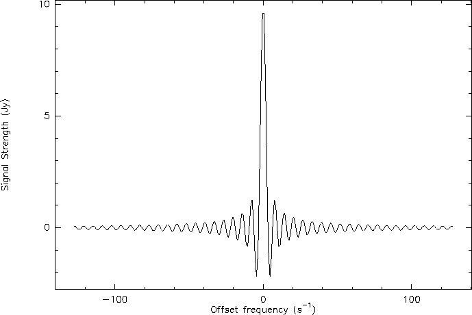Figure 1: The X-Window graphic window just before clearing the plot in the demonstration procedure.

 

10.

This command not only clears the graphic screen, but also destroys the current drawing. A new empty window is re-created afterwards.

 

11.

Define the values of the X and Y coordinates at the corners of the plot window. Here, manual setting is used for X axis, and automatic setting for Y axis.

 

12.

Define the type of marker you want. A marker is a regular polygon defined by its number of summits (0 to infinite), the type of polygon (0 to 4) and diameter in physical units (which on a paper output will be centimeters). Try the different values for the type to see what it means.

 

13.

Now, plot a marker as defined above at each data point. Note that you do not need to read again your data, neither to define again the user coordinates, the last values have been retained.

 

14.

and connect the data points by a smooth curve.

 

15.

Read data into the Z buffer from column 3. You need not redefine the data file, neither the line range which are the same as in command number 2. The Z buffer is similar to the X and Y arrays into GreG but used in different ways.

 

16.

Use the values in the Z buffer to draw symmetric error bars along the Y axis at each data point. The Z values will define the length of each side of the bar in Y user coordinates.

17.

Same effect as above, but since the plot has been cleared...

18.

idem...

19.

idem...

20.

Specify the text centering mode

21.

write some legend to the figure

 

22.

This plot seems good, make a hardcopy to save it. With the option /PLOT the command sends the hardcopy to the default system printer. This command has many other possibilities, such as creating PostScript files. Your plot should look like figure 2.

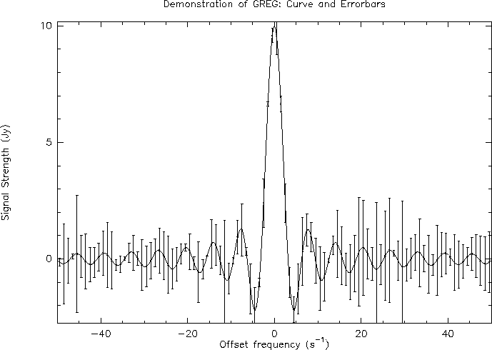Figure 2: the printed output of the simple demonstration procedure.

You have now mastered most of the 1 dimensional capabilities. At this point, you may want to add some title or any other comment on your plot. Then you will need to get a hardcopy of your drawing and to send it to a plotter.